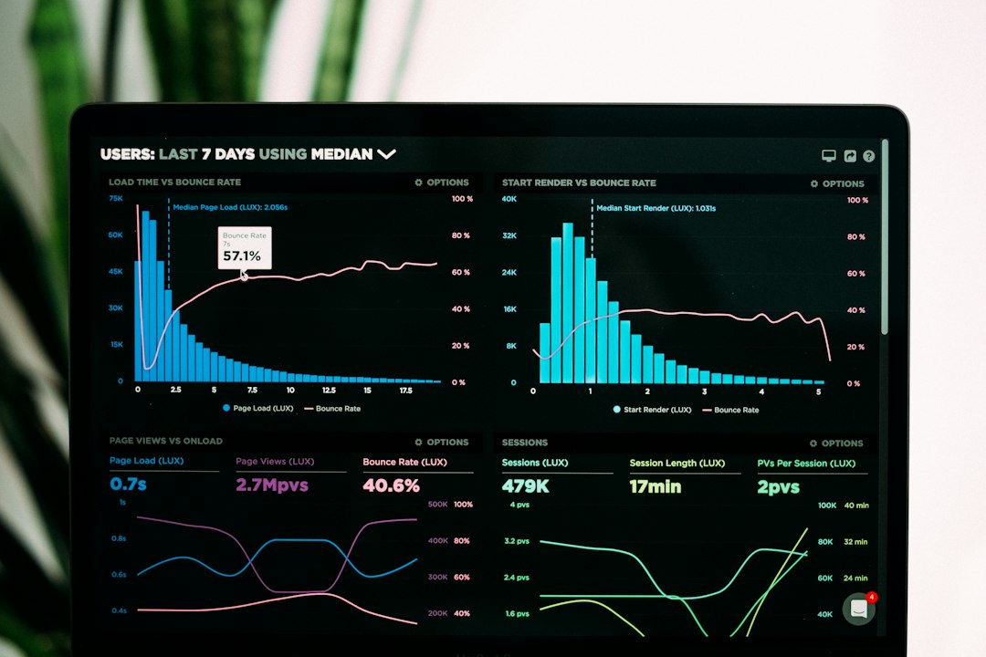
Photo by Luke Chesser on Unsplash
Continuous Profiling: Always-On Visibility Into What Your Code Actually Does
Traditional profiling is a detective’s tool: something goes wrong, you suspect a bottleneck, you reproduce it, attach a profiler, collect data, and investigate. This workflow has a fundamental flaw — production behavior is often impossible to reproduce in a controlled setting. Continuous profiling fixes this by collecting lightweight performance data all the time, building a historical record of where CPU time actually goes.
How Sampling Profilers Work
Continuous profilers are almost universally sampling-based. Rather than instrumenting every function call — which is prohibitively expensive — they interrupt the CPU at regular intervals, typically around 99 Hz, record the current call stack, and resume execution. After thousands of samples, patterns emerge: functions that appear frequently are consuming the most CPU time.
The key technical challenge is stack unwinding — reading the call stack at the moment of interruption. In compiled languages with frame pointers, this is straightforward: each stack frame holds a pointer to the caller’s frame, so you walk up the chain. But modern compilers often omit frame pointers as an optimization. Alternatives include DWARF debug info (expensive to parse at runtime), compact unwind tables baked into the binary, or hardware-assisted unwinding via features like x86’s Last Branch Record.
eBPF has made in-kernel profiling substantially more practical. A profiler can run an eBPF program in the kernel’s perf subsystem, capturing stacks with minimal context before handing them off to a userspace consumer for symbolization and aggregation. This approach keeps the hot path lean and defers the expensive work.
The Overhead Question
The practical barrier to always-on profiling has always been cost. A naive instrumented profiler can slow a program by 2–10×. Sampling at 99 Hz with an eBPF-based implementation typically adds less than 1% CPU overhead — acceptable for most production workloads.
The remaining cost is symbolization: translating raw instruction addresses to function names and source locations. This can be deferred. The profiler stores raw addresses in a ring buffer, then resolves symbols in a background process or at query time. You trade a modest amount of memory for CPU headroom on the hot path — a reasonable tradeoff for observability infrastructure.
Flamegraphs and Differential Analysis
The standard visualization for profiling data is the flamegraph. Each horizontal bar represents a function; its width represents the proportion of samples in which it appeared; the call stack grows upward. Functions with wide, flat tops — a wide bar with no children wider than a sliver — are where time is actually spent. Deep narrow stacks represent common call paths that aren’t expensive.
Continuous profiling adds a dimension single-shot flamegraphs lack: time. By comparing profiles between two time windows or two software versions, you get a differential flamegraph showing which functions got slower or faster. This is how you verify that a code change actually improved production performance, not just a microbenchmark.
Where Profiling Fits in the Observability Stack
Metrics, logs, and traces are the canonical three pillars of observability. Profiling is increasingly described as a fourth, and the distinction is meaningful. Metrics tell you that latency increased. Traces tell you which request was slow. Profiling tells you why — down to the specific function consuming CPU.
The integration story is still maturing. OpenTelemetry has a profiling signal in active development, which would let profiling data flow through the same collection pipeline as traces and metrics. The compelling use case is correlating a trace span with CPU samples from the same time window: not just how long a request took, but exactly where within that request the CPU time went.
Challenges in Heterogeneous Environments
Continuous profiling is well-understood for single-language compiled services. It gets harder in mixed environments. Managed runtimes — JVM, V8, CLR — have their own internal stacks that a kernel-level profiler can’t see without runtime cooperation. The JVM exposes hooks like AsyncGetCallTrace specifically for this purpose; tools like async-profiler use them to reconstruct application-level frames. Interpreted code gives you interpreter frames, not meaningful application frames. Mixed-mode stacks, where native code calls into managed code or vice versa, require stitching together multiple unwinding strategies without double-counting frames.
Runtime vendors have been gradually adding better profiler support as demand has grown, so the polyglot picture is improving.
The Shift in Mindset
The deeper change continuous profiling enables is moving performance work from reactive to proactive. Instead of waiting for an incident to hunt down a bottleneck, teams can review CPU trends as part of normal development. A regression introduced on Tuesday shows up in the continuous profile long before it manifests as a latency alert — which is the point. Observability tools are most valuable when they surface problems before users do.